Inductive Thinking#
When we are using deductive logic we take facts and use them to deduce new facts. This is a very powerful practice. We say that by adding first order logic we can start talking about more general concepts, like all integers.
The process of inductive reasoning is a method of looking at a subset of observations at drawing a general conclusion. You do this constantly. As humans, we often cannot explicity test all possible situations. Instead, we look at some information and generalize the information.
When you take a new class, you probably expect that there will be some negative consequence of submitting work late. You may be wrong, but in many cases your prediction is correct. You have created a generalization about all classes based on your experience in some classes.
This idea is the basis for inductive reasoning. In this case, your inductive reasoning is informal. You are making a generalization, but it might not be right. You have limited information and make your best generalization.
With formal inductive reasoning we will make generalizations that must be true for the situation in question. The critical difference will be how we verify our observations generalize.
Concepts#
Assume your friend has a bag of jelly beans at their house. They tell you that there are exactly 100 jelly beans in the bag. The bag is solid and you cannot see inside. You take out 4 jelly beans to eat. They are colored: red, red, yellow, green.
Your friend asks you to guess how many of each color are left in the bag. Based on your life experience, you might guess the colors are roughly uniform in their distribution. This means the handful you took was a reasonable sample.
You make a prediction:
50% of 96 jelly beans are red (48 red jelly beans)
25% of 96 jelly beans are yellow (24 yellow jelly beans)
25% of 96 jelly beans are green (24 green jelly beans)
Your friend opens the bag and you find out that a dozen of the jelly beans are blue. You realize there was information you were missing!
Your guess was made using inductive reasoning. You had a set of base cases. A base case is a specific point of data we know the answer to. You knew the answer for 4 jelly beans exactly. You took them out of the bag. Your reasoning was solid so far.
Next, you made a inductive hypothesis. You assumed that your example data predicted accurately the remaining jelly beans. This hypothesis was based purely on your own life experience eating jelly beans. This is the point where you reasoning could either succeed or fail. If you made a good hypothesis, you would predict the correct answer. If you made a flawed hypothesis you would predict the wrong answer.
You generalized the information you had to the jelly beans you didn’t know about. The problem is that your generalization wasn’t anything that could be proven conclusively ahead of time. You just made an educated guess.
In a formal Proof by Induction, we will need some reasoning to justify why our data can actually be generalized.
Turing Complete Programming Languages#
in 1936, Alan Turing invented a concept called the Turing Machine [Hod12]. A Turing Machine is a very simple computer that can do anything that a computer can do [Tur37a]. Turing proved that any algorithm that can be run on a general purposed computer can be run on a Turing Machine. This was used to create the concept of Turing Completeness. Any program that can simulate a Turing Machine can run any algorithm a general purpose computer can.
The difference between the jelly bean guess and Turing work is the confidence about the generalization. It is certain that any programming language that can simulate a Turing Machine can run any algorithm a general purpose computer can. This generalization is much stronger then guess that jelly beans are uniformly distributed.
We can still use inductive reasoning in this case. Let us assume you have a Python program and you want to know if it can be translated to Racket. You could translate the code yourself and do a single experiment. Then you might guess that based on your experience a different Python program could actually be translated. You might be right, but you might be wrong.
We could determine the generalization with certainty. We could implement a Turing Machine in both Python and Racket. We could then use Turing work to say that since a Turing Machine can run any algorithm a general purpose computer can, we can translate any Python program into Racket. We know for certain that the two programming languages can do the same set of tasks.
We still needed one program that worked on both systems, the Turing Machine Simulator. We just made a must stronger generalization. This was because we had a definative prediction about programming languages provided to us by Alan Turing.
Binary Decision Tree#
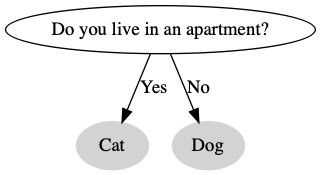
Computer programs often used a concept called a decision tree. A decision tree is a collection of questions that is used to make a decision. At the top of the tree is the root. This is the first question we ask. At the bottom of the tree, we have leaves. These are the results of the decision tree.
We want to make a program that predicts what pet you should get. The first question we ask is if you live in a house of apartment. We will suggest that cats are better pets for an apartment.
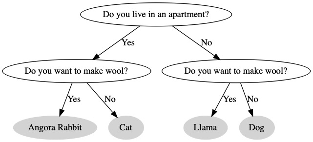
If we want to ask a second question, we need to add it to both paths. Now, we have four leaf nodes. We don’t make a decision until we ask all the questions.
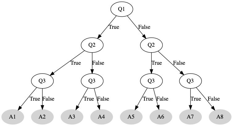
Each of our questions is a yes/no. We can change this to a true/false boolean. For each question we ask, we will set a variable to be true or false depending on the result. Then our answers are the leaf nodes. If we have 3 questions we need to ask, there are a total of 8 possible answer. We need to come up with a different answer for each situation.
We want to generalize this concept as follows:
A binary decision tree with \(v\) variables will have \(n\) leaf nodes where \(n = 2^{v}\).
Base Cases#
We have already created a number of base cases we can refer back to. A base case is a specific instance of the problem we know the answer to. (In the next section, we will further formalize these concepts).
Number of Variables |
Number of Leaves |
|---|---|
1 |
2 |
2 |
4 |
3 |
8 |
Inductive Hypothesis#
We need to come up with a way to generalize our base cases to any tree. We know that for \(1 \le v \le 3\) the formula works. We are going to assume it works for larger values. We aren’t sure of this. Think back to deduction. Sometimes when we assumed something it lead to a useful conclusion. Other times, it lead us to a contradiction.
Let us assume for any number of variables in the range \(1 \le v \le X\) the following formula holds
\( \begin{align} n = 2^{v} \end{align} \)
We know this formula works when \(X=3\). We are just assuming it would work for \(X=4\) or \(X=5\). We don’t know that yet.
Inductive Case#
Let us assume we have a decision tree with \(X\) variables. By our hypothesis, we know how many leaf nodes the tree will have.
\( \begin{align} n = 2^{X} \end{align} \)
What happens if we added one more variable to this decision tree? Every existing leaf node is now one question away from a final answer. Each of the previous leaf nodes need to ask one more boolean question. This means the new number of leaf nodes must double \(2*n\).
\( \begin{align} 2n =& 2*(2^{X}) \\ 2n =& 2^{X+1} \end{align} \)
The number of variables in the new decision tree is \(X+1\) it is one greater than the previous number. The number of leaf nodes as doubled. We doubled the values on both sides of the expression.
If the formula held for \(X\) then it does hold for \(X+1\). We completed this by reasoning about the tree structure, but in the next section we will see how to formally complete this type of reasoning.
Proof by Induction#
We knew from our experiments that \(n = 2^{v}\) was true for the range \(1 \le v \le 3\). Our inductive case shows that if the statement was true for a range, it was also true for a range one larger. That means \(1 \le v \le 4\) must be true. Once we know that, we also know a range one larger is true. That means \(1 \le v \le 5\). This pattern goes on forever.
\( \begin{align} \forall v \in \{1 \le v \le 3\} (n = 2^{v}) \implies& \forall v \in \{1 \le v \le 4\} (n = 2^{v}) \\ \implies& \forall v \in \{1 \le v \le 5\} (n = 2^{v}) \\ \implies& \forall v \in \{1 \le v \le 6\} (n = 2^{v}) \\ \implies& \cdots \\ \implies& \forall v \in \{1 \le v \le \infty\} (n = 2^{v}) \end{align} \)
Since our inductive hypothesis was completed with a general range, we can keep using it over and over again. We can conclude that the formula work for all natural numbers.
Conclusion#
In this section, we saw how we can generalize a concept to a large group using only information about a small group of test elements and reasoning. In the next section, we will look at Mathematical Induction which will formalize this process into a proof method. We will no longer have any guess. We will be able to write out a formal mathematical proof that will be either correct or incorrect.