
FOL Rules#
When we combine Boolean Logic, Predicates, and Quantifiers, we are in a new system. This system is called First Order Logic (FOL). It is called first order because only inputs to functions are variables. There is also a concept of High Order Logic, where functions can take other functions as inputs.
Compressed Notation#
If we want to reason about expressions, they can become very complex to write. We can state that a number is either even or odd. A number that is not even must be odd.
\( \begin{align} \forall x \in \mathbb{Z} \left( \text{even}(x) \vee \neg \text{even}(x) \right) \end{align} \)
This is very easy to read, but if we were to use it in a proof by deduction things could get messy. We need to remember to write the \(\mathbb{Z}\) on every time. We also need to keep writing \(\text{even(x)}\) and matching all our parenthesis.
To make proofs easier, there is a standard method for making compressed expressions. We compress the expression to do the proof. Then expand our conclusion again at the end.
The rules are as follows:
If all variables come from the same set, we can drop it.
All variables must be one lowercase letter.
All functions must be one uppercase letter.
Drop all predicate input commas and parenthesis.
We rewrite out above statement in compressed notation as
\( \begin{align} \forall x \left( Ex \vee \neg Ex \right) \end{align} \)
Imagine we wanted to define a predicate to check if integer \(g\) is the Greatest Common Denominator (GCD) of integers \(a\) and \(b\).
What does it mean for a number to be a GCD? It must be the largest number that evenly divides both values.
We want to create a predicate GCD that takes three inputs \(a\), \(b\), and \(g\). It returns true if \(g\) is in fact the GCD of \(a\) and \(b\).
First, we need a way to determine if two numbers divide each other. This can be done with the remainder, but we will define a shorter name. The predicate \(R\), for remainder zero. It returns true if \(\frac{x}{y}\) has no remainder.
\( \begin{align} Rxy := (x\%y \equiv 0) \end{align} \)
We know the GCD must divide both inputs. We can start our predicate there.
\( \begin{align} GCD(a,b,g) := Rag \wedge Rbg \cdots \end{align} \)
The value \(g\) must all be the \(largest\) number that makes this true. For all other numbers, if that number is a common denominator, it must be less that or equal to \(g\). We introduce a new variable \(x\). If \(x\) is not a common denominator, we don’t care about it. If it is a common denominator, it must be less than or equal to \(g\). This is a great application of the conditional. We only care about common denominators.
We need a new predicate to handle less than or equals to.
\( \begin{align} Lxy = x \le y \end{align} \)
We put all the pieces together to get a full expression.
\( \begin{align} GCD(a,b,g) := Rag \wedge Rbg \wedge \forall x \left( (Rax \wedge Rbx) \implies Lxg \right) \end{align} \)
We could write this without the compact notation, but it takes up more space.
\( \begin{align} GCD(a,b,g) := (a \% g \equiv 0) \wedge (b \% g \equiv 0) \wedge \forall x \in \mathbb{Z} \left( ( (a \% x \equiv 0) \wedge (b \% x \equiv 0) \implies (x \le g) \right) \end{align} \)
Using this version in the proofs shown below would add a significant amount of extra writing and more chances to make mistakes.
This statement has two types of variables. There are bound variables and free variables. The bound variables are tied to a quantifier. In this example, there is one bound variable called \(x\). It is bound in the sense that it must meet the requirements of the quantifier.
The expression has three free variables. These variables are not tied to a quantifier. They can be set to any value. The predicate will return true or false depending on the setting of the free variables.
We can use this expression as a road map to implement the function. In practice, it would be easier to just compute the GCD and compare our answer to \(g\). This is done as an example of converting a FOL statement into code.
In a practical situation, we would be making a function like this to test a different function. For example, we could use it to verify Euclid’s algorithm on a number of tests.
#Implement a test based on predicate logic
def GCD(a,b,g):
    result = True
    #Remainder of a and g must be 0
    result = result and (a%g==0)
    #Remainder of b and g must be 0
    result = result and (b%g==0)
    #For all x until max(a,b)
    #All larger numbers can't have a remainder of 0
    for x in range(1,max(a,b)+1):
        conjunction = ((a%x)==0) and (b%x==0)
        #Uses or def of implies
        implies = not (conjunction) or (x <= g)
        #Combine with result
        result = result and implies
    return result
#Find the GCD by Trial and error using our function
def GCD_by_test(a,b):
    for g in range(1,max(a,b)+1):
        if GCD(a,b,g):
            return g
    return -1#Error Case

#Implement Euclid's Algorithm
def euclid(a,b):
    if b==0:
        return a
    else:
        return euclid(b,a%b)

#Test our Code on random numbers
import random
if __name__=="__main__":
    random.seed()
    a=random.randint(2,100)
    b=random.randint(2,100)
    print("Computing GCD of",a,"and",b)
    g1=GCD_by_test(a,b)
    print("Trial and Error Found:",g1)
    g2=euclid(a,b)
    print("Euclid's algorithm Found:",g2)
    if g1==g2:
        print("Answers Match!")
    else:
        print("Error: Answers Different")
Both methods find the same answer.
Computing GCD of 63 and 70
Trial and Error Found: 7
Euclid's algorithm Found: 7
Answers Match!
We will see later that trial and error is sometimes the best solution, but this is very infrequent. The advantage of this kind of trial and error is to give us a check to confirm a more efficient algorithm is correct. We also also use to to help debug that algorithm or verify properties of that algorithm.
Interpretations#
If we have an expression written in a compressed notation, we may need to expand it. Sometimes, it will not be obvious what functions or variables mean. The process of assigning meaning to the symbols is called interpretations.
A statement that is true for one interpretation may be false for a different interpretation. In practice, we will always have some information to interpret based on. Frequently, source code or text commentary. Then we just have to match symbols together.
Imagine we had the following expression.
\( \begin{align} \forall x,y,z \in \mathbb{N} \left( (Pxy \wedge Pyz) \implies Pxz \right) \end{align} \)
If we define \(P(a,b):= a \le b\) then this statement is true and makes sense.
\( \begin{align} \forall x,y,z \in \mathbb{N} \left( ((x \le y) \wedge (y \le z) ) \implies (x \le z) \right) \end{align} \)
If \(x\) is less than or equal to \(y\) and \(y\) is less than or equal to \(z\), then we can determine that \(x \le z\) must be true.
On the other hand, if we define \(P(a,b):= a \neq b\), the statement makes no sense.
\( \begin{align} \forall x,y,z \in \mathbb{N} \left( ((x \neq y) \wedge (y \neq z) ) \implies (x \neq z) \right) \end{align} \)
This statement can be easily made false. We pick \(x=5, y=7, z=5\).
\( \begin{align} ((5 \neq 7) \wedge (7 \neq 5) ) \implies (5 \neq 5) = \text{False} \end{align} \)
The fact that two numbers are different doesn’t get us the same implies. Even though we will be working with pure symbols for the rest of this section, remember that they must have underlying meanings. Our focus for now is on the rules themselves, but once our context expands interpretations will become much more important.
For All Rules#
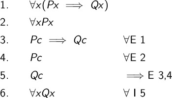
There are two rules related to the for all quantifier. If we know something is true for all values, we can make up a constant. It will be true for that constant. This is the for all elimination rule. If we reach a conclusion with a constant that has no assumptions related to it, then it doesn’t matter what that constant’s value was. The statement must be true for any value. This is the for all introduction rule.
We show these in the following example. We prove the following argument.
\( \begin{align} \forall x (Px \implies Qx), \forall x Px \therefore \forall x Qx \end{align} \)
The basic idea for the proof is that we assume there is some constant \(c\). Since the statements are true for all values, they must hold for this specific \(c\). We then complete a standard proof by deduction. Since the proof held for whatever \(c\) we picked, it must be true for any value. We never needed to know anything about the \(c\) we picked.
Exists Rules#
When working with exists, we need subproofs. The statement is not true for every value. We can only assume that we can find at least one value that makes the statement true.
We will show the exists introduction and exists elimination rules through an example. We prove the following argument.
\( \begin{align} \forall x (Qx \implies Rx), \exists x (Px \wedge Qx) \therefore \exists x (Px \wedge Rx) \end{align} \)
The basic idea of this proof is that we assume we found the value that exists. We call it \(c\). Then we use this value to prove other statements are true. Each line is described in more detail below the proof.
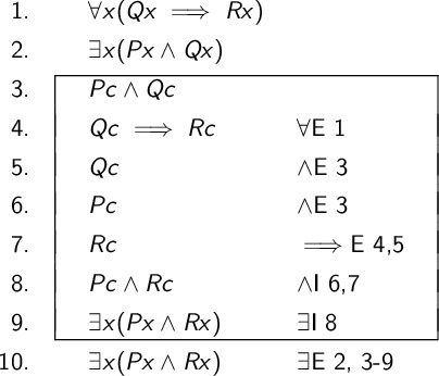
We start with a premise.
We include the second premise.
Based on premise 2, we can assume there is a constant \(c\) that makes \(Pc \wedge Qc\) true. We are imaging we found the value somehow.
The implies must hold for the \(c\) we found, since it holds for everything.
We take apart the conjunction.
We continue taking apart the conjunction.
The implies tells us that if \(c\) makes \(Q\) return true, it also makes \(R\) return true.
We combine two statements we know to be true.
If this \(c\) constant we imagined actually exists, then it also makes \(Pc \wedge Rc\) true. Within the assumption, there does exist a way to make this statement true. It is the \(c\) we imagined.
We imagined that a constant \(c\) existed. In this line, we confirm that wasn’t an work of our imagination. We actually know for a fact (from line 2) that a value does exist. So, our subproof was a reasonable assumption and we can draw conclusions from it.
Conversion of Quantifiers#
There is an extension of the Demorgan Laws for quantifiers. Just like with classical logic, the quantifier flip when a negation is applied.
\( \begin{align} \neg \forall x Px \iff& \exists x \neg Px \\ \neg \exists x Px \iff& \forall x \neg Px \\ \end{align} \)
Since these are bi-conditionals, we need to prove both directions. These rules are called the Conversion of Quantifiers or CQ for short. They are Derived Ruled because, as shown in the following proofs, we can build them from the basic rules.
For All#
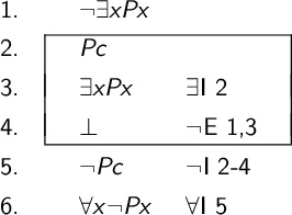
The first argument we prove is \(\neg \forall x Px \therefore \exists x \neg Px\). The general approach here is to assume \(\neg \exists x \neg Px\). There does not exists any value that makes the statement false. By contradicting this, we prove that there must be at least one value that makes \(Px\) false.
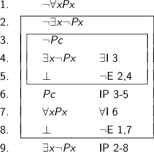
The steps are explained in more detail below.
We start with the premise.
We assume there cannot exist any value that makes \(Px\) false.
We assume that we found a value \(c\) that makes \(Pc\) false.
We state that since we found \(c\), at least one value must exist.
We create a contradiction. We said that a solution exists and also no solution exists.
If no value can make \(Px\) false, then it must for true for \(Pc\)
Since \(c\) could be any value, we can say for all.
This is also a contradiction with the premise.
We conclude that the assumption \(\neg \exists x \neg Px\) must have been false.
The second direction is has the conclusion and premise flipped. We prove the argument \(\exists x \neg Px \therefore \neg \forall x Px\). The general approach is to prove that \(P\) cannot return true for all inputs under this premise. The steps are detailed below the proof.
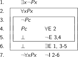
We start with the premise.
We assume \(Px\) is true for every value.
We assume there exists a value \(c\) that cause \(P\) to return false.
Using the for all, we know \(c\) makes \(P\) return true.
There is a contradiction, \(P\) cannot return two different results on the same input.
We know that there exists a value that makes \(P\) false from the premise, so the \(c\) we assumed does exists. We can move the contradiction out of the subproof.
We conclude that it was impossible for \(P\) to return true for all inputs.
Exists#
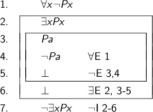
To prove \(\neg \exists x Px \iff \forall x \neg Px\) we start with the argument \(\neg \exists x Px \therefore \forall x \neg Px\). The approach is to assume there exists some value that makes \(P\) return true. Then prove this is impossible.
We start with the premise.
We assume there is a value \(c\) that causes \(P\) to return true.
This means there exists at least one value that makes \(P\) return true. (Hint: It is \(c\).)
This contradicts the premise which said no values existed that made \(P\) return true.
If nothing makes it true, then it must be false.
There is nothing that can make \(P\) true, so it must be false for all inputs.
The last argument to prove is \(\forall x \neg Px \therefore \neg \exists x Px\). We assume that there exists at least one value that makes the predicate return true. This is impossible, which means there cannot exist anything that makes the predicate true.
We start with the premise.
Assume there exists at least one value that makes \(P\) true.
Assume that value is named \(a\).
We know from the premise that \(a\) will make \(P\) return false.
We contradicted, a predicate cannot return two values on one input.
We assumed that at least one value existed, so we can pull out the contradiction.
We contradicted the existence of any value that makes \(P\) true. One cannot exist.
Invalid FOL Statements#
Just like with boolean logic, a FOL statement can be invalid. If we prove a statment true, then it is true for all interpretations.
To show something is invalid, it just needs to be invalid for one interpretation. This is a little more work that with boolean values, because we still need to define a set and predicates.
Is the statement \(\exists x \in S (Px) \therefore \forall x \in S (Px)\) valid or invalid?
This statement is invalid. We can give two examples. Either one would be enough.
In many cases, you will find a math based example is easiest. There is nothing special about math, but you probably know a lot of rules already. That will help you come up with examples.
We define the set \(S=\{1,2,3\}\). We define \(Px\) to be true when \(x\) is even. The premise is true. The expression \(\exists x \in S (Px)\) is true since \(2\) is even and found in \(S\). The conclusion \(\forall x \in S (Px)\) is false. There are two numbers in our set \(1\) and \(3\) that are not even. We conclude this argument is invalid.
To show a FOL argument is invalid, you need to meet a few requirements.
Define your model, the elements in the set and definition of predicates.
Show that your premises are all true in your model.
Show that your conclusion is false in your model.
There may be other models where the conclusion is true. If we change the above set to \(S=\{2,4,6\}\) the conclusion would hold. An argument is only invalid if it always holds. Just holding on some examples is not good enough.
We can provide a second invalid argument without using numbers.
Let \(S\) be a set of animals. We have \(S=\{ \text{crow}, \text{rabbit}, \text{dog} \}\). Let the predicate \(Px\) be true if \(x\) is a bird. The premise is true. The expression \(\exists x \in S (Px)\) is true since the crow is a bird and found in \(S\). The conclusion \(\forall x \in S (Px)\) is false. There are two animals in our set rabbit and dog that are not birds. We conclude this argument is invalid.
Proving arguments are valid requires a full proof. Proving something is invalid just requires one example that shows a situation were the premises are true and the conclusion is false.